part of a basin of attraction of a value v=4,
neighborhood k=3, size n=9, 1d cellular
automaton, with the nodes shown in 2d.
Below: the color scheme for v=4 cell values.
complex kcode with many emerging gliders, glider
guns, and self-replicating structures, on hex
lattice. Click to enlarge, click here for info.
1d n=150 v=8 k=5 k-totalistic Altenberg rule,
where lookup table entries are set according
to a probability which depends on the frequency
of colors in each neighborhood. This example
was filtered to emphasise gliders. Click to enlarge.
Discrete Dynamics Lab

Update Nov 2005

(revised from previous updates Dec 04 and Sept 04)

DDLab Version m05: multi value logic, totalistic rules, many new features

return to: DDLab home - DD-Life - Multi-Value examples

The most significant changes since the last binary release:

Multi-value DDLab includes many other new features, improvements and revisions, both major and minor, since the last official release in May 2002. Some of these, but not all, are listed below. The usual harvest of bugs have also been fixed (and not too may added - we hope!).

For previous updates since March 96,
click Dec 03, July 01, Feb 99, Sept 97.

Some new features and changes


Forward only for just totalistic rules


complex kcode with emerging spirals on hex lattice. click to enlarge, click here for info

Multi-value logic


Totalistic and outer-totalistic rules

The updated prompts for totalistic and outer-totalistic rules are as follows...


2d neighborhoods (square and hex) updated

As mentioned earlier, the max neighborhood size when DDLab is constrained to run forward-only, for just totalistic rules, is k=25 (for v>5 k is reduced). For the full lookup table, max-k=13 (for v>3 k is also reduced).

The predefined 2d neighborhoods have been extended up to k=25 on a square and hex lattice. The layouts try to achieve a reasonable symmetry, which is not always possible. Only the symmetric neighbourhoods are shown below, defaults have a black background. If square and hex are equally symmetric, square is the default. The asymmetric layouts not shown can still be selected.
To force hex for any k there is a new option in the top right WIRING prompt.

Below are the predefined fully or partly symmetric neighborhoods. (defaults with a black background).
Note that the center cell may form part of its neighborhood, or not. If it does it is shown in red.

k=4 k=5 k=6 k=7 k=8 k=9 k=10 k=11 k=12 k=13 k=14 k=15
square
lattice
hex
lattice

k=16 k=17 k=18 k=19 k=20 k=21 k=22 k=23 k=24 k=25
square
lattice
hex
lattice


Toggling between square and hex presentation

In the 2d wiring graphic prompts, there is a new prompt, This toggles the lattice presentation between hex and square, changes the highlighted cell's neighborhood to a local CA predefined neighborhood, and toggles the neighborhood between hex and square (if possible).

In the "on the fly" prompts when running forward in 2d, there is a new prompt to change between square or hex presentation,

For CA with a square neighborhood, the 2d space-time pattern will start on a square lattice, if hex on a hex lattice.

Setting rules/states updated


Classification of rule-space and complex rule sample

The automatic classification of rule space has been updated for multi-value. Samples of glider/complex rules are available that can be randomly set on-the-fly when running forward, with g,
These files are in dd_extra.tar.gz and include the following,

rule sample automatic classification files:

  • for 1d, v=2, full lookup table, as before but renamed,
    • v2k5ss.sta (k=5)
    • v2k6ss.sta (k=6)
    • v2k6ss.sta (k=7)
  • for 1d, multi_value, full lookup table,
    • v3k3ss.sta (v=3 k=3)
    • v4k2ss.sta (v=4 k=2)
    • v4k3ss.sta (v=4 k=3)
    • v5k2ss.sta (v=5 k=2)
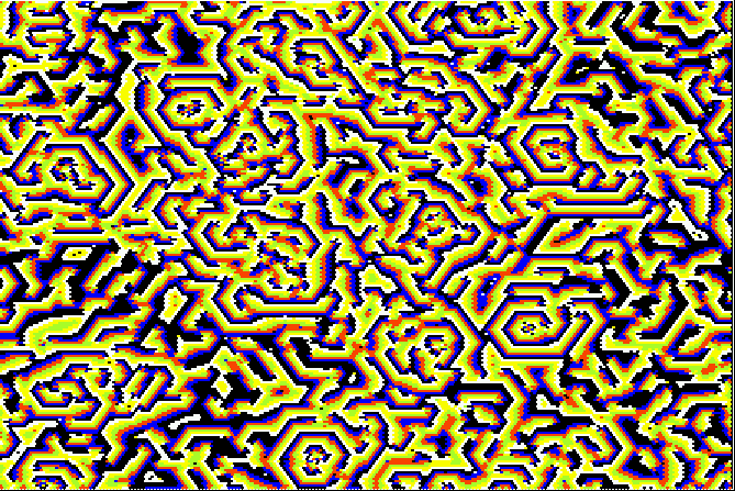
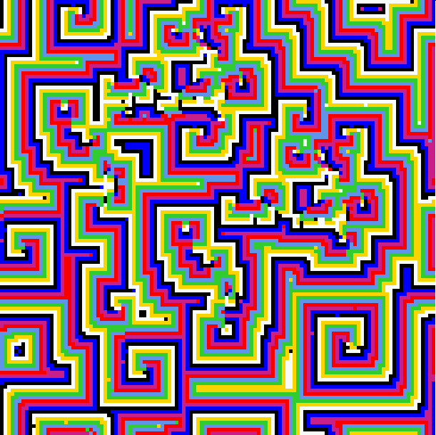
  • for 2d, multi-valye kcode,
    • v3k4bs.sta (v=3 k=4)
    • v3k5bs.sta (v=3 k=5)
    • v3k6bs.sta (v=3 k=6)
    • v3k7bs.sta (v=3 k=7)
    • v4k4bs.sta (v=4 k=4)
    • v4k6bs.sta (v=4 k=6)
glider/complex rule sample files for loaded on-the-fly with "g":
  • for 1d, v=2, full lookup table, as before but renamed,
    • g_v2k5.r_s (k=5)
    • g_v2k6.r_s (k=6)
    • g_v2k7.r_s (k=7)
  • for 1d, multi_value, full lookup table,
    • g_v3k3.r_s (v=3 k=3)
    • g_v3k4.r_s (v=3 k=4)
    • g_v4k2.r_s (v=4 k=2)
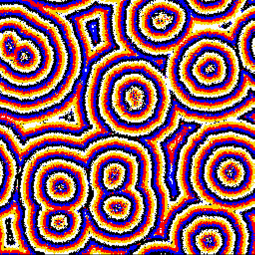
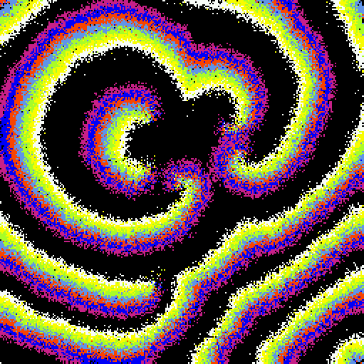
  • for 2d/3d, kcode lookup table,
    • g_v3k6.r_v (v=3 k=6)

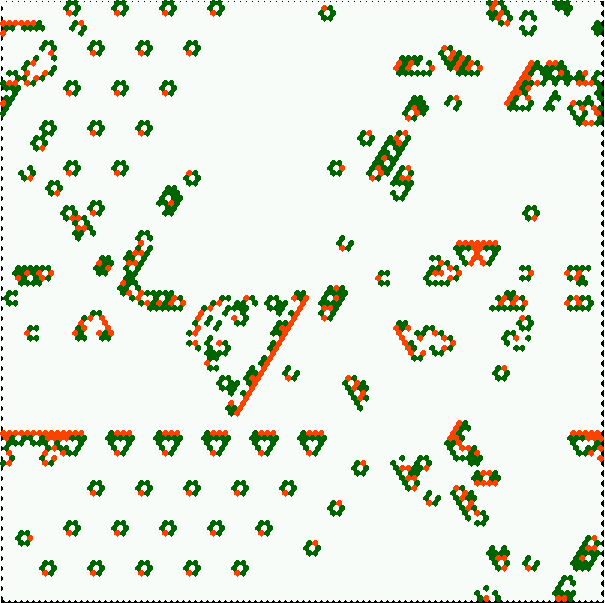
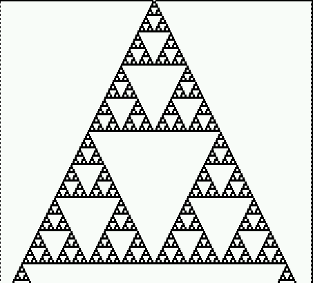
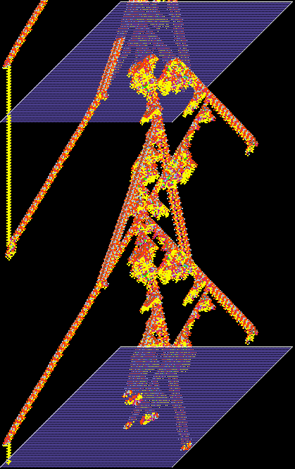
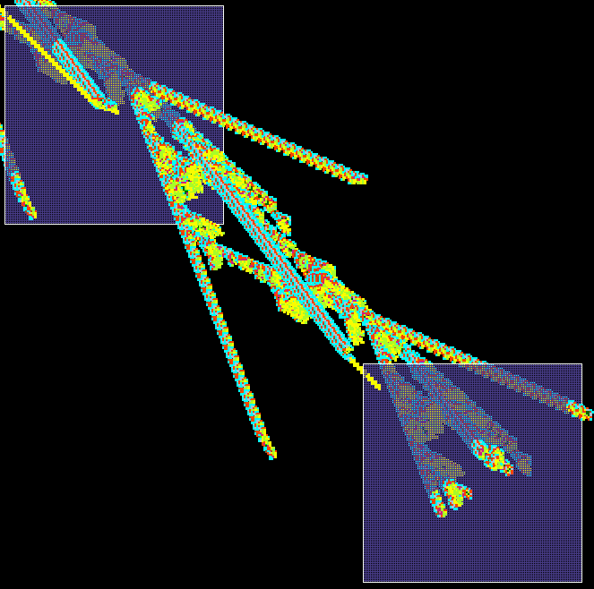
An automatically classified sample of about 16000 v=3 k=6 kcode rules for 2d hex CA
Axies are as follows:
x=standard deviation of the input-entropy, y=mean entropy, z=frequency of rules on the xy scatter plot.
Complex rules are spread out on the right with higher standard deviation, Chaotic and ordered rules are on the left with low standard deviation - chaos has high entropy (the tower), and order lower entropy.


The "un-slant" option, rule 153, Click to enlarge.

New/revised on-the-fly options

When running forward, there are some new and revised on-the-fly options as follows:

rules

presentation change seed size presentation

Falling of edge boundary conditions

By default, the boundary condition in DDLab are periodic, a ring for 1d, a torus for 2d and a 3d torus for 3d. There is a new option, in the top right space-time pattern interrupt options, to set a fixed border of a given value and width. If a suitable border width, and border value (same as the background), are set, gliders and other structures in 2d and 3d complex CA can seem to fall of the edge, simulating an infinite space, though structures sometimes interact with the edge.


Scrolling 2d space-time patterns

The basic 2d pattern can be transformed on-the-fly into two different kinds of space-time patterns (axonometric projections), and both can be scrolled for a continuous view of the unfolding of the dynamical system (click to enlarge).
The system shown is a complex kcode CA on a hex lattice, with two glider guns. These glider guns oscillate between the firing of gliders in opposite directions.


above:
the basic (default) 2d presentation

right:
starting with the basic 2d presentation, enter 't' to project a vertical axonometric, as if looking up into a shaft (an old option). A new option makes the pattern scroll when reaches the bottom of the screen; enter "#" to toggle scrolling on/off.


above:
starting with the basic 2d presentation, enter "#" to project a diagonal axonometric, which will automatically scroll when it reaches the bottom of the screen; enter "#" to toggle between basic 2d and this presentation.


Reaction-Diffusion Dynamics, Excitable Media

Reaction-Diffusion dynamics [Greenberg and Hastings] is made with a CA consisting of 3 types of cell: resting, excited, and refractory. There is usually one resting type, one excited type, and one or more refractory types. A resting cell becomes excited if there is a threshold, or threshold interval (t) of exited cells within its neighborhood. An excited type changes to refractory. A refractory type changes to the next refractory type (if there are more than one) and the final refractory type changes back to resting, completing the cycle. The resulting dynamics produces waves and spirals and related patterns that can resemble the BZ reaction and other types of excitable media. The dynamics depends on the initial state and its density of non-resting types - usually low for best results. Reaction-Diffusion dynamics can also be produced with a locally wired random network, where each cell has random inputs from a local zone. In DDLab Reaction-Diffusion can be set as an "outer" k-totalystic rule, or as a full lookup table.

In the first method, select outer k-totalystic, as described in section Forward only for just totalistic rules

As a full lookup table, at the prompt for selecting a rule, enter R (... RD-R ...). Note that max v/k allowed is smaller than with the outer k-totalystic rule method.


Reaction-Diffusion on a 222x222 hex grid k=12, v=6:
0 rest, 1 excited, 2 to 6 refractory. The threshold interval is 5 to 6.
Reaction-Diffusion on a 122x122 square grid k=8, v=8: 0 rest, 1 excited, 2 to 6 refractory. The threshold interval is 1 to 6. Non-resting density about 30%

Reaction-Diffusion on a 255x255 square grid,
v=5: 0 rest, 1 excited, 2 to 5 refractory. The threshold interval is 3 to 15. k=24 random connections within a 12 cell diameter local zone.
Reaction-Diffusion on a 255x255 square grid k=11,
v=8: 0 rest, 1 excited, 2 to 11 refractory. The threshold interval is 2 to 7. k=11 random connections within a 12 cell diameter local zone.


Return to the Discrete Dynamics Lab home page.
Last modified: Sept 2005